Big Muff Pi emulation

[Fire Sledge - Ohm Force]

Hi everybody

I’m currently modeling a Big Muff Pi fuzz stompbox. More exactly, the one I’ve got at hand, a “Green Russian Tall Font” version. It was my first guitar pedal back in the 90’s and it’s still in a relatively good shape. I would need some help or advices form experimented people here, but first I’m going to present the details of this project. Just tell me if I did something wrong.



My goal is to use the emulation on a Raspberry Pi 4 which is the audio processor of my own pedalboard. I’m not sure if it will have enough processing power to manage the BMP along with other effects, but I’ll try.

Of course the results or products I would come up with will be free and open source, so feel free to reuse or modify anything. For the circuit simulation, I’ve set up a nodal DK-method program. More on this later.

The BMP input stage is of quite low impedance for a guitar device, so the output impedance of the previous element in the chain (a guitar, another pedal or buffer) may have a significant effect on the sound. I deliberately chosen to use low-output impedance signals (as the one coming from a buffer) for all the measurements and simulations. The reason is that there are as many different output impedances as different guitars, and it seems that people generally don’t find much difference in the BMP tone with or without buffer, unlike some other fuzz pedals like the Fuzzface.


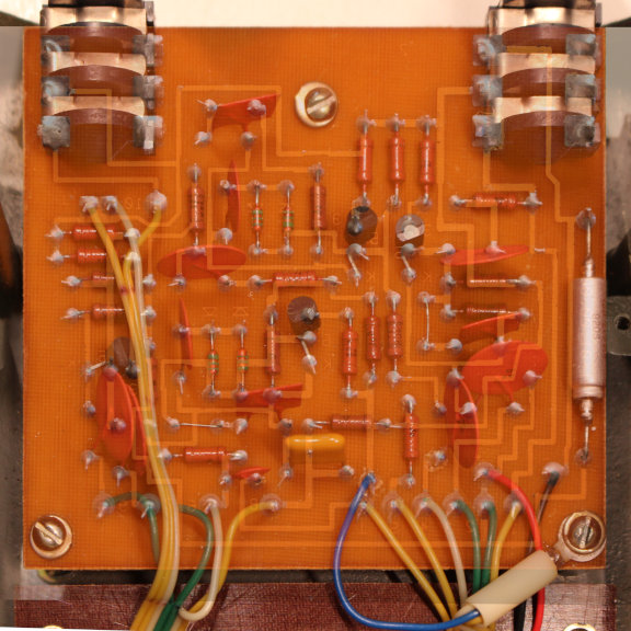
Overlaying pictures of both sides of the PCB helps to identify the parts

I did some initial measurements. I ran a test signal through the pedal and recorded it at different points in the circuit. I repeated with different settings. Recording were done with an audio interface, a Fireface UCX. To minimize any perturbation on the BMP and saturation on the interface side, I built a high impedance buffer and attenuator and inserted it between the measurement point and the audio interface input. It is not totally transparent (there’s a -90 dB rumble from its power supply), but it should be OK. Recording were done in 24 bits 88.2 kHz. Input signal is about 1 V of nominal amplitude (2 V peak-to-peak), and repeated at -20, -40 and -60 dB. It is made of a 10-octave sweeping sine and some other waveforms (saws in both directions and square). I think this covers most of I need to achieve a decent emulation. I probably could have done this with my oscilloscope but I think this way is more convenient.



Measurements can be downloaded here. Files are named with the three knob values (d = distortion, t = tone, v = volume) from 0 (CCW) to 1 (CW) and the measurement point (q2c = transistor Q2 collector). There is also the buffer recorded alone, for scaling purpose and to check the whole recording chain perturbations (noise, mains hum, DC removal, etc).

I also read the bias voltages for all transistors:

Code: Select all

        Q4       Q3      Q2       Q1
V_C   4.60     4.42    4.74     5.70
V_B   0.756    0.749   0.739    1.517
V_E   0.1515   0.154   0.1329   0.928

The battery voltage was between 9.25 and 9.18 V.

I modeled the whole circuit according to this schematics. There are some minor differences, the base-collector feedback caps are single 510 pF (with wires on the second cap locations), and the transistors are labelled “EE1”. The pots are labelled “CП4-2M D7 18T 150K” excepted for volume with D9 instead of D7, so I guess they are 150 kΩ.

The DK-method simulation runs way too slowly at the moment, but it is a lesser concern for now. The results are quite close to the SPICE one, but not close enough from the original. Of course, it was expected. Now I’m trying to tweak the model, stage by stage, to match the BMP as close as possible. This is where I need some help.

I’m working on the input stage. I modified some resistor and capacitor values so it reacts well. But I stumble on something I don’t understand. With low signals (-40 dB, the third one, starting at 3:27 on the measurement samples), the original BMP input stage exhibits some light distortion, with almost only odd hamonics. The SPICE simulation does the same, but mine has all the harmonics (and probably too much of them). I tried to tweak the part parameters to no avail. I use simple stateless models for the diodes and transistors (Shockley and Ebers-Moll), so I guess the difference comes from here. But before I try to implement much more complex models like Gummel-Poon, anyone has an idea about what could cause the small-signal distortion to be more or less symmetrical instead of asymmetrical?

Thank you, sorry to be a bit long

[DaveClark]

Hi,

I would expect something simpler causing that particular problem, such as a sign error in your derivations and/or code you've written. I can't imagine how use of Ebers-Moll instead of Gummel-Poon would cause that problem, but it's been a long time since I've worked with transistor models, especially bipolar. In fact I would say that if changing to Gummel-Poon somehow got everything working, you still probably had a sign error!

Regards,
Dave Clark

[Fire Sledge - Ohm Force]

Thank you very much for your reply! It solved my issue.

I quadruple-checked the formulas and the code, but found nothing wrong. However it reminded me to check the precision. Indeed, when I started circuit simulation with the MNA, it was quite clear to me that over a few nodes, double precision was absolutely required. When I switched to the DK method, I found that single precision didn’t cause the convergence issues I previously encountered and I settled to float data.

Then I just checked with double precision and shazam! the even harmonics are gone. Using double will possibly worsen my CPU load issue (or not, if it speeds up convergence as with the MNA), but I’ll see this later. Now I can continue tuning the model.

[mystran]

Fast methods like LU (and inverting the matrix is even worse) for solving the linear algebra (ie. the MNA matrix equation) are usually not ideal in terms of numerical precision so using double precision is always a good idea. In some cases you additionally rely on small "fudge factors" like gMin conductances that would have to be made unreasonably large if you wanted to work in single-precision. In other cases you could get away with single-precision by switching to a numerically more stable solver, but this is likely to cost you a lot more performance than just using doubles.

[Fire Sledge - Ohm Force]

Yes, that’s what I figured out.

I’ve got quite decent results now. I still have a few corner cases like square wave input in the 20–30 Hz range being a bit too much defined, so it needs more finetuning. But the overall sound is convincing. Waveforms and spectrum match relatively well and I couldn’t really tell the difference with the real thing on an actual guitar input.

Code: Select all

Nodes      :  26
Voltage src:   2
Pots       :   6
Energy st  :  13
Non-linear :  10
Output     :   1
Simulating...
Speed:       62.886 kspl/s (x1.426 real-time).
=== Iterations ===
Average: 2.58
  1:      13384,   0.6 % #
  2:    1285197,  54.9 % ################################################################
  3:     829151,  35.4 % #########################################
  4:     145534,   6.2 % #######
  5:      29339,   1.3 % #
  6:      18768,   0.8 % #
  7:      13635,   0.6 % #
  8:       3904,   0.2 %
  9:         96,   0.0 %
 28:          1,   0.0 %

This is without oversampling (edit: and without moving any pot), on a standard RPi4. It needs optimization now to be usable as a real-time effect, before refining the sound.

[Ivan_C]

Have a look for the DAFX15 article about Newton-Raphson's method improvements too, and don't forget that oversampling might reduce the number of needed iterations to get convergence

[Fire Sledge - Ohm Force]

Have a look for the DAFX15 article about Newton-Raphson's method improvements too

Thanks for the pointer. I more or less paused my DSP learning and research activities for a long decade and came back at it a few months ago, so I still have a huge pile of DAFx papers and concepts to catch up. I think the article you’re mentioning is Improving the robustness of the iterative solver in state-space modelling of guitar distortion circuitry. I’ll check it in detail. I already do rough step capping, but the article seems to present something more sophisticated.

and don't forget that oversampling might reduce the number of needed iterations to get convergence

Definitely. However the overall CPU load still increases with the oversampling rate.

The profiler tells me that:
– 92 % of the time is spent in the non-linear part of the solver, including:
– 47 % in the jacobian LU decomposition
– 23 % in the pre-multiplication of the jacobian with the K matrix
– only 4 % in the non-linear i(v) evaluations, which are not even SIMD parallelized yet.

I’m not sure at which point the matrix operations can be sped up; once multiplied with the K matrix, the jacobian is no longer sparse (although it looks quite symmetrical, I don’t know if there is a way to take advantage of it [edit: it’s the K matrix which is symmetrical, not the jacobian]). So I guess I have to first find a way to reduce the number of calls to the LU decomp.

[DaveClark]

Hi Fire,

Have you considered the impact of a user such as yourself rapidly changing parameters during a simulation? This is what steered me away from N-R, LU, etc. approaches for real-time.

I would be interested in hearing about people's experiences, i.e. the impact on re-factoring, how to handle previous solutions, etc. as parameters are quickly changed. For example, a user can instantly change a 250K ohm potentiometer to nearly zero, then immediately change another 1M ohm potentiometer from nearly zero to 1M ohm, with the result that the ratio covers many orders of magnitude as the changes are being made. The optimum setup for solution could be drastically different for the beginning and endpoints, also dynamic while it's all happening.

Thanks for any war stories!

Regards,
Dave Clark

[Fire Sledge - Ohm Force]

I haven’t done extensive tests, but it seems that a 10 kHz full range potentiometer modulation increases the average number of iterations to around 18 (vs 3–4 with constant parameters, higher than normal input signal and no oversampling) for my BMP model. I think this is not a big deal as you usually don’t change parameters at such a high and sustained rate, excepted for some specific use like audio-rate modulation of a filter cutoff frequency for example. Sparse abrupt changes have sparse impacts on the convergence. And you can smooth the parameter changes anyway. Lower audio rates have less or no significant impact on the convergence.

An interesting thing about the DK method described in Physical Modelling of a Wah-wah Effect Pedal as a Case Study for Application of the Nodal DK Method to Circuits with Variable Parts is the separation between the variable and constant resistors. When variable resistors change, you only have to invert a small matrix based on theses resistors, not the full system.

[mystran]

The profiler tells me that:
– 92 % of the time is spent in the non-linear part of the solver, including:
– 47 % in the jacobian LU decomposition
– 23 % in the pre-multiplication of the jacobian with the K matrix
– only 4 % in the non-linear i(v) evaluations, which are not even SIMD parallelized yet.

I’m not sure at which point the matrix operations can be sped up; once multiplied with the K matrix, the jacobian is no longer sparse (although it looks quite symmetrical, I don’t know if there is a way to take advantage of it). So I guess I have to first find a way to reduce the number of calls to the LU decomp.

You don't want to call a LU decomposition function, you want to inline the whole thing. You don't even want to store the matrix inside an array, you want to store all the (non-zero) components as separate variables to make sure they get the best possible register allocation.

Also whenever you have a matrix where some dimensions are linear while others are non-linear (and hence need to be updated every iteration) you want to pivot the matrix in such a way that you can do a partial LU decomposition of the linear dimensions before you even enter the iteration loop. You can then start each iteration from this state, add the varying conductances and just finish the decomposition for the dimensions that where actually changed.

In fact, a naive MNA matrix has a ton of dimensions that are (1) completely constant and (2) you don't really care for the final value. In this case, you can similarly do a partial LU decomposition for just those dimensions and then throw them away completely at compile time.

So basically, if you are solving more than one dimension per capacitor or input/output (or variable resistor) in the outer loop, or more than one dimensions per bipolar junction in the inner loop, then you certainly can optimize the code. And I want to repeat: don't store matrices, but rather unroll the whole thing, it'll give you a big (probably like an order of magnitude) speedup.

[Fire Sledge - Ohm Force]

That’s why the DK method is nice: it formalizes what you described. The outer loop is just made of a few matrix-vector products. Non-linearities are isolated so the inner loop can focus on solving the voltages or currents at the junctions. Contributions from the other parts of the circuit is just a vector to add to the function to solve. If there are 10 junctions, the jacobian to decompose is 10×10.

Edit: basically the outer loop looks like this:

Code: Select all

p   = h * u + g * x;
i_n = solve_nl (p, k);
v_o = e * u + d * x + f * i_n;
x   = b * u + a * x + c * i_n;

where v_o contains the desired output voltages, x the energy-storage component states, u the input voltages and i_n the non-linear currents found in the inner loop using p as contribution from the other parts of the circuit. Matrices a to k are built from the MNA description of the circuit and assumed dense and constant.

[urosh]

BTW, you can decompose BMP into 4 independent blocks run is series, where biggest inaccuracy in model would be loss of nonlinear loading of first clipping stage. Output buffer could be replaced with linear stage as well, and you could even put all potentiometers "outside" of solver, or at least two (tone pot and output attenuator)

[Fire Sledge - Ohm Force]

I tried it, but the sound was quite different. My initial idea—if it had worked—was to use a common structure for the 4 stages and parallelize the processing with SIMD, at the cost of a 3-sample delay on the final output. Maybe I messed up something and should give it another try. I used simple fake loads trying to mimic the impedance of the previous/next stages in small signals (2nd order filters). BTW the last stage is more than an output buffer, it has some gain and distorts, especially when the tone pot is turned counterclockwise the input signal may have a large swing. But you’re right, the last volume pot could be externalized.

[urosh]

You have to include whole tone control into second clipping stage model, but you can get away without tone potentiometar (replace ti with resistor and calculate voltages at the ends of that resistor)

edit: that's if you want to exclude variable resistors from models. Certainly more accurate would be to include tone potentiometer, and replace final stage with capacitor and resistor, to simulate final stage loading on tone control network.

[DaveClark]

When variable resistors change, you only have to invert a small matrix based on theses resistors, not the full system.

Hi Fire,

Thanks for that insight.

Regards,
Dave Clark